
Phase and time alignment
- Product Code: Real-Time Analyzer (RTA)
- Availability: 2-3 Days
Explanation of the various RTA functions
Real Time Analyzer – RTAThe real-time analyzer is an essential instrument for the precise adjustment of a DSP device. In its current version, the RTA is a perfect aid – both for those who want to adjust their sound system in the least possible time and for sound enthusiasts who want to carry out high-precision measurements with great care.
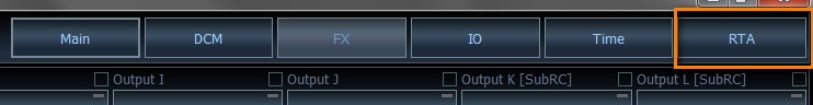
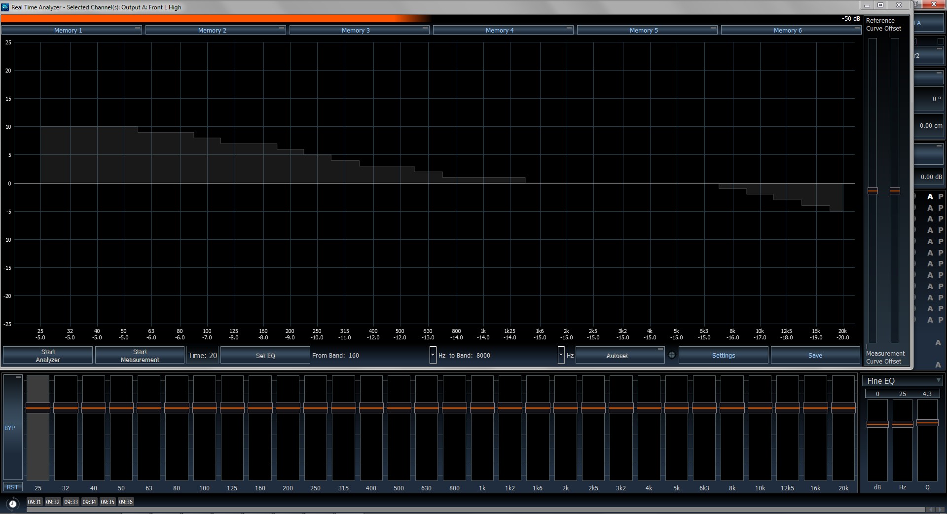
1. Starting the RTASimply click on the marked “RTA” button to open the RTA menu:
 If you operate the DSP PC-Tool in demo mode, the analyzer will not work. Only when you connect one of our DSP components to your computer the analyzer will offer its full range of functions and allow measurements. The equalizer remains visible as an overlay even when the RTA menu is opened and its size can be scaled so that it can be placed above the EQ sliders; means that the RTA's measuring bands are exactly "aligned" with the EQ bands which considerably simplifies the operation.
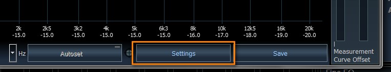
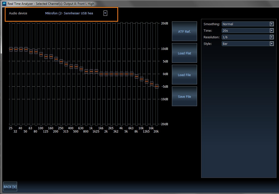
2. General settingsBefore working with the RTA, you must check the general settings. You can access the corresponding menu by clicking the "Settings" button:
2.1. Choosing the reference curveSelect the desired reference curve for adjusting the equalizer and the filters in the DSP. The "ATF Ref." is always predefined as a standard, since this curve is also used in industry for the calibration of cars. Alternatively, you can select a linear (“Load flat”) reference curve. This curve should only be used for home applications and not for measurements inside a vehicle, since in the latter case it will not lead to satisfactory acoustic results. If the ATF reference curve does not suit your taste, you can also define your own curve. Each frequency band can be changed individually for this purpose. Save a self-defined reference curve on your hard drive using “Save File” so that you can recall it at a later date using “Load File”.2.2. SmoothingThe amplitude response is the result of many individual measurement points over a certain time span that are "smoothed" into a curve. This smoothing takes some time to generate a "constant" display. With "fast" smoothing, the time can be reduced, but at the expense of the measurement accuracy in the lower frequency range. A "slow" smoothing only makes sense if the highest accuracy is required in connection with a long measurement duration. The default value "normal" should be the best choice in most cases.2.3. Measurement duration (Time)While measuring the amplitude response, the microphone has to be moved back and forth in a semicircle between the left and right ear. In the meantime, the RTA records a large number of measurement points, which are integrated into a constant display over the measurement time. In order to obtain accurate and reproducible measurement values, a minimum measurement duration is required, which should not be less than 10 seconds. The measuring accuracy increases with increasing measurement duration. The standard value of 20 seconds has proven to be the perfect compromise between expenditure of time and accuracy.2.4. ResolutionA frequency resolution of the RTA in 1/3 octave steps is set by default. This resolution is very practical because it reflects the human hearing impression very well. For this reason, an amplitude response measured in 1/3 octave steps and smoothed in the same resolution by the equalizer usually leads to a pleasant sound characteristic. However, if the result is not satisfactory, it can be worthwhile to increase the resolution of the RTA in order to detect narrow-band flaws in the amplitude response. The hearing is quite “immune” to narrow-band dips, but reacts quite sensitive to narrow-band peaks, which mostly are the result of resonances. When you flatten the frequency response you should focus primarily on eliminating these peaks. Narrow-band dips are mostly the result of cancellations due to phase errors, which cannot be corrected at all or only inadequately with the equalizer.2.5 StyleBoth the reference curve and the measurement curve can be displayed in different ways. The practicable bar graph is defined as default. Alternatively, the curves can also be displayed as lines or as "impulses".3. Sound pressure displaySufficient sound pressure level of the test signal is essential to achieve a proper measurement result. The RTA uses a coloured bar in the upper area to indicate whether the level of test signal is sufficient for the measurement or not.Green bar All dB values between -30 dB and 0 dB are shown as a green bar. In this case the sound pressure level is sufficiently high for a measurement.
3.1 Adjusting the right sound pressure level
Advice: You have to carry out the adjustment of the sound pressure level again for each vehicle and for each individual calibration position. 4. Starting the analyzer and a measurementAs soon as you click on the "Start Analyzer" button, the current measured value of the measurement microphone is displayed as a “red” curve. The graph is quite unsteady at low frequencies, so that a correct reading of the amplitude response is difficult. It is therefore necessary to carry out an integration over a large number of measurement points which happens when you click the "Start measurement" button. All measured values are now averaged over the set measuring duration – indicated by the white curve, which will be automatically “frozen" after the measuring time has elapsed.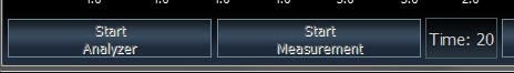 If you want to compare this measurement with later readings, it makes sense to save it temporarily. Simply click with the right button of your PC mouse on the key button of the desired memory location (Memory 1 - Memory 6). The measurement curve of each storage location is shown in a different colour for better differentiation: Memory 1: red curve Memory 2: dark blue curve Memory 3: green curve Memory 4: yellow curve Memory 5: pink curve Memory 6: light blue curve Important: The content of the memory 1 - 6 is lost after closing the DSP PC-Tool. If you want to save a measurement permanently for later documentation purposes, use the "Save" button at the bottom right of the display. This allows you to save the complete display content of the RTA as a png file. 5. Shifting the measurement curve and the reference curveFor both the manual equalization and the AutoSet function, it is essential that the measurement curve and the reference curve are superimposed in a meaningful way.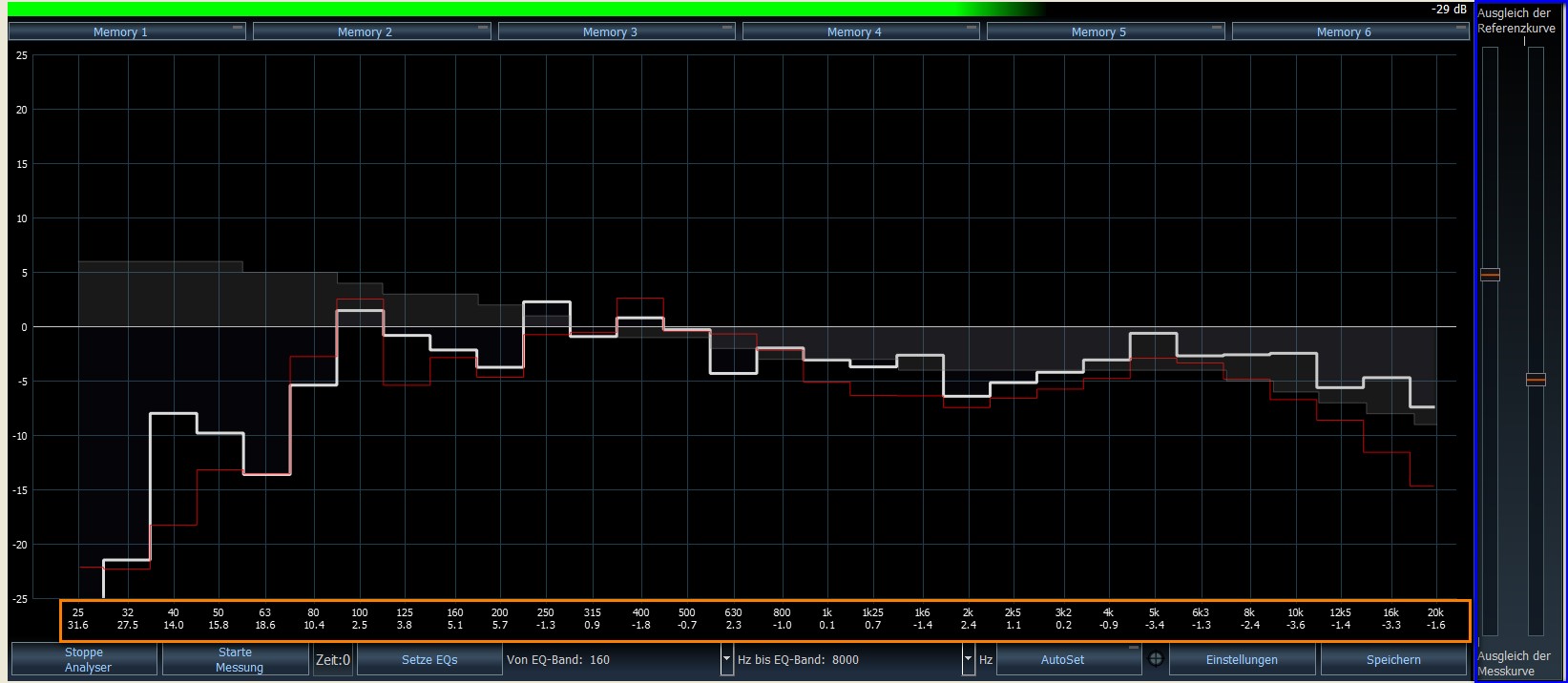 The curves can be “moved” using the two sliders on the far right of the RTA display (marked in blue). Which of the two sliders you use is up to you. However, it is always useful when both curves are positioned in the center of the display or slightly above. We recommend shifting the reference curve in such a way that the “difference” between the two curves shows more peaks than dips. To make this adjustment more convenient, the difference between the measurement curve and the reference curve is displayed in dB values below each EQ band (highlighted in orange). Positive values correspond to the necessary boosts in the respective bands, negative values require corresponding cuts. Be careful with strong boosts (> 4 dB), as this can easily lead to overdriving of the DSP and thus a drastic increase in distortion. On the other hand, strong cuts (-10 dB or more) are possible without any problems. Advice: Even if you increase the resolution of the RTA to 1/6 octave or higher, only the offset values for the 1/3 octave resolution are displayed. 6. The SetEQ and AutoEQ featuresOf course you can manually transfer the differences between the measurement curve and the reference curve to the equalizer, but this is much more convenient using the "SetEQ" function. If you click the "Set EQs" button after the measurement, all equalizer bands will be adjusted in the frequency range that was defined with the two drop-down menus: Even if it seems tempting to have the full audio frequency range from 25 Hz to 20,000 Hz automatically adjusted, you should be cautious especially if there are large deviations between the measurement and reference curve. Because then it may happen that critical boost values are transferred to the equalizer, which, as described above, can lead to either strong distortion and/or an increased noise level. After executing "Set EQ", start the measurement again in order to check how well the measurement curve and the reference curve now match. Usually there are still some deviations after the first cycle, so that "SetEQ" has to be processed again. With each further iteration step, the measurement curve and reference curve should converge better. If you are not interested in the individual optimization steps, you can use the particularly convenient "AutoEQ" function instead of "SetEQ". A measurement followed by a calibration of the equalizer are automatically carried out alternately one after the other. If the measurement and reference curves do not converge even after several cycles, an error message will appear: 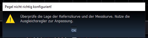 |


 & Input EQ")
